BIOL 297: Class project analyzing COVID-19 pandemic data

Description

In response to moving the course online, I have decided to combine the final project and exam into a larger project that will be 35% of your final grade. As decided in class, everyone will analyze by, themselves or with a partner, a dataset to test a hypothesis that could explain why COVID-19 has spread more rapidly in some US states than others. This page is a placeholder for further information on this project. I will notify you via email when I make important updates.

Learning objectives

• translate questions and scientific hypotheses into testable statistical hypotheses
• synthesize data from online sources
• analyze data using a null hypothesis testing framework
• draw appropriate conclusions
• communicate quantitative information effectively through written and visual media

What you must turn in by classtime (12 PM) on Thursday, May 14

The R script and analyses are worth 75% of your final project grade; the written and oral presentations are worth 25%.

• R script and data files to perform all analyses (see explanation and example)

• Blog-style report for lay readers (~3 paragraphs)

• Presentation to class using slides (~5-10 minutes)

The report and presentation should be understandable by a lay audience without specialized biological or statistic background. The report and presentation must address all of the following elements to receive full credit:

1. Motivate your study (e.g. this could be based on an observation, a new report, or some kind of hypothesis you were interested in testing)
2. Pose your question
3. Describe your data and where you obtained them from
4. Describe the statistical method you used to address your question
5. Describe your results using appropriate figures and/or tables (you can use or modify the figures from your R report)
6. Based on your analysis, what do you conclude?
7. Address 1 or 2 limitations of your analysis. In particular, you must describe a sampling bias and/or confounding variable that might have caused you to reach the wrong conclusion. If you fail to reject your null hypothesis, you can also describe how the statisical power of your study was limited, in which case you should refer to the confidence intervals on your parameter estimate.

Each element can be described briefly in a couple sentences. You don’t need to provide detailed background or citations.

Timeline:

• Friday, April 10: One paragraph proposal of scientific question and hypothesis

• Friday, April 24: Get all data you will need to complete project

• Friday, May 1: Data analysis plan due. Step-by-step explanation below on how to complete this on RStudio Cloud. If you want, you can work on a local project and email it to me.

  • Create project on RStudio Cloud. Call it “last-first-final” (e.g. “muir-chris-final”). You can simply click “New Project”; you don’t need to import GitHub Repo, as in labs.

• If necessary, move data files into project directory using the upload tool. Once files are uploaded, you will see them in your Files tab:

• If you need to get data entered into a CSV files, look at Section 2.6 in the textbook called “How to make data files” for guidance.

• Create new R script for your code.

• Install any packages you need.

• In script, complete a draft of the “Question”, “Hypotheses”, and “Test you will use” sections, as in the example final. It would look like:

• Thursday, May 14

  • R script and data files to perform all analyses (see explanation and example)
  • Blog-style report for lay readers due
  • Online symposium of results with 5-10 minute presentations

Getting started

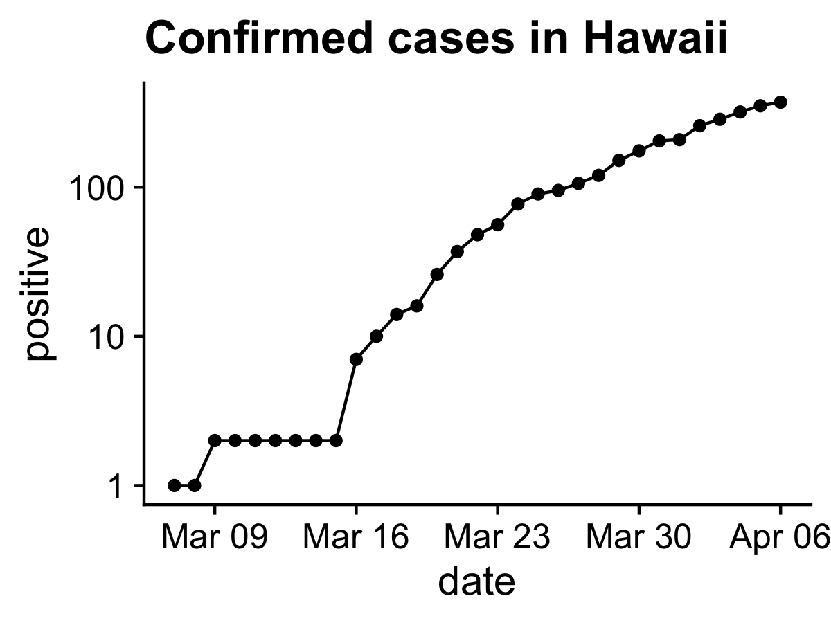
You can look at up-to-date data from the COVID Tracking Project by copying and pasting the code below into R. You should get a figure like the one below. Notice this code uses some nifty R functions we haven’t encountered yet, like the pipe operator %>% and mutate(). Read about them and try to understand what they do (I use them all the time).

library(cowplot)
library(lubridate)
library(tidyverse)

covid <- read_csv(
  "https://covidtracking.com/api/states/daily.csv", 
  col_types = cols(
    date = col_character(),
    state = col_character(),
    positive = col_double(),
    negative = col_double(),
    pending = col_double(),
    hospitalized = col_double(),
    death = col_double(),
    total = col_double(),
    hash = col_character(),
    dateChecked = col_datetime(format = ""),
    totalTestResults = col_double(),
    fips = col_character(),
    deathIncrease = col_double(),
    hospitalizedIncrease = col_double(),
    negativeIncrease = col_double(),
    positiveIncrease = col_double(),
    totalTestResultsIncrease = col_double()
  )
) %>%
  mutate(date = ymd(date))

covid %>%
  filter(state == "HI") %>%
  ggplot(aes(date, positive)) +
  scale_y_log10() +
  geom_line() +
  geom_point() +
  theme_cowplot()